
Exploring Tiling - Part 1 - Geohash
Introduction - Why Tiling?
Let’s say we have data spread throughout Seattle (e.g. housing sales, school grades or ratings, number of restaurants, etc). We want to aggregate that data into easier to understand pieces. Let’s say you started with a polygon outlining the City of Seattle (KC data source). Below are two version of the Seattle outline. One is a screenshot of the raw file in QGIS, the other is a geopandas plot using the following:
city_df = gpd.read_file("/python_r_comp/admin_SHP/admin/city.shp")
fig, ax = plt.subplots(figsize=(5,12))
#there are multiple cities King County `city.shp` dataset
city_of_interest = 'Seattle'
single_city = city_df[city_df['CITYNAME']==city_of_interest].copy()
#change coordinate reference systems to be compatible with other datasets
single_city.to_crs({'init': 'epsg:4326'}, inplace=True)
single_city.plot(color='none',
                   edgecolor='black',
                   legend=True,
                  ax=ax)

_ = single_city.apply(lambda x: ax.annotate(s=x['CITYNAME'],
                                           xy=(x.geometry.centroid.x,
                                               x.geometry.centroid.y), ha='center'),axis=1)
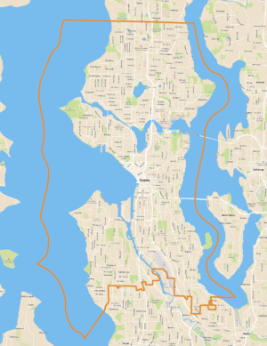
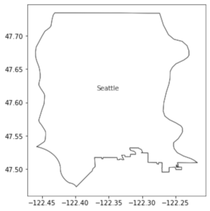
Above (left) Seattle boundary with a basemap and (right) Seattle boundary without a basemap from geopandas
A good starting point for aggregating data across Seattle would be to separate the Seattle polygon into into neighborhoods based on the King County neighborhood dataset (dataset source). The neighborhood dataset looks like this:
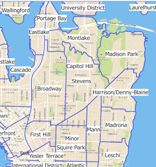
You could easily aggregate data by neighborhood and the neighborhood names would be recognizable by the end user of your analysis. But, a major drawback is the inconsistent nature of political or social boundaries like neighborhood. Neighorhood boundaries provided by King County can change and so can the names. Some sub-neighborhood groups can develop or recede.
A more consistent political/social boundary is the Census Bureau Blocks or Block Groups (gov website link). US Census Bureau tries very hard to maintain consistency with Blocks and Block Groups so year-over-year analysis should be straightforward and you can incorporate Census results into your data analysis. This is a pretty promising approach. The drawbacks with using Blocks or Block Groups is that they were created to a) split up inhabitable land (i.e. there are no Groups on lakes or rivers), and b) they have been optimized for population surveying not necessarily for the type of analysis you’re performing. The last drawback to using any social or political boundary is that you don’t have a consistent spatial or geometrical relationship between neighbors.
In order to get consistent neighbor relationships, we’ll have to set our sights on tiling methods and tile geometries.
Tiling
In general, there are three geometries that easily tile: rectangle, triangle, and hexagon.
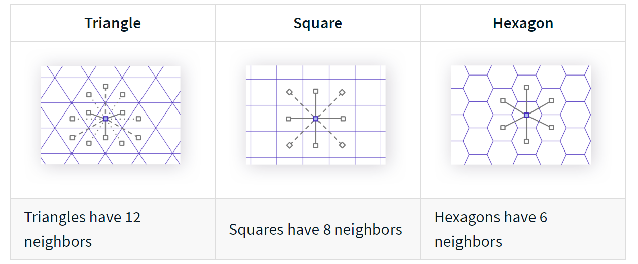 Grid layouts from uber’s H3- hexagon tiling documentation
You can see from the Uber graphic above, there are some unique benefits to hexagons that I’ll cover in another post - for now, we’re focusing on rectangles. One way to create a consistent rectangle grid is to use a geohash grid. A helpful website for understanding the levels of geohashing is this interactive-geohash.
Here’s a static image from that site of the earth broken down into geohashes:

As you can see from the image above, there are various scales of geohash rectangles, created in order to cover the whole globe. Each rectangle grid can be broken into smaller rectangles. From the image, you can see the g rectangle is broken up into gh, gk, gs, gu, etc. There’s a ton of information on the wikipedia page about the specifics of making the grid and the geohash characters but I want to focus on two benefits for breaking up large datasets:
- consistency
- not spatial
Consistency
Creating a grid from a geohash library like Python’s geolib will always return the same geohash and boundaries given the same 3 inputs:
- latitude
- longitude
- precision (or scale)
from geolib import geohash
geohash = geohash.encode(latitude, longitude, precision=6)
Every geohash has a pre-defined bounding box. For instance:
latitude = 47.64495849609375
longitude = -122.3712158203125
precision = 6
test_geohash = geohash.encode(latitude, longitude, precision)
#geohash = 'c22zp3'
bounds = geohash.bounds(upperleft_geohash)
#bounds = Bounds(sw=SouthWest(lat=47.6422119140625,
#                           lon=-122.376708984375),
#                ne=NorthEast(lat=47.647705078125,
#                            lon=-122.36572265625))
Once you pick a scale the geohash rectangle grid will be consistent no matter what data you’re using as the input. Here’s a close up of the geohash grid in Seattle with a precision of 6. The rectangle c22zp3 is highlighted in red.
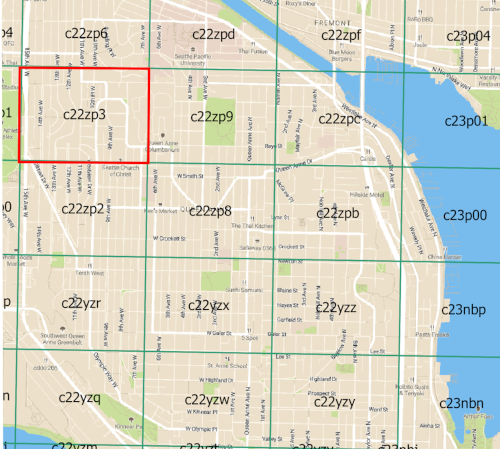
Any latitude and longitude that falls into the geohash rectangles bounding box will always be encoded with the geohash c22zp3 at precision=6.
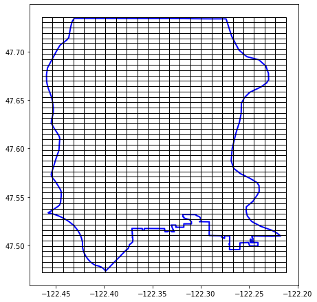
Here’s a picture of the geohash grid on top of the Seattle boundary polygon (below).
To illustrate the importance of the consistency with a geohash grid. I’ll show you another way to create a grid. Instead of using geohash rectangles, you can break the Seattle polygon into pieces using open street map Python library’s function quadrant_cut_geometry (h.t. blob reference for showing me this option). The below code snippet breaks the Seattle polygon into quadrat_width=0.01 which is ~1000 m in ESPG:4326 (aka WGS84, which has units in degrees).
# make the geometry a multipolygon if it's not already
geometry = single_city['geometry'].iloc[0]
if isinstance(geometry, Polygon):
  geometry = MultiPolygon([geometry])
geometry_cut = ox.quadrat_cut_geometry(geometry,
                                        quadrat_width=0.01)
seattle_cut = gpd.GeoDataFrame(crs={'init':'4326'}
                 ,geometry=[geom for geom in geometry_cut.geoms])
The image below is created by just plotting seattle_cut: seattle_cut.plot()
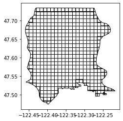
You can see that the grid seems similar to geohashing rectangles and it has the benefit of being very customized for your polygon or area of interest. The customization comes at the cost of consistency and it can have some buggy effects near the corners (as you can see in the picture above). Similar to neighborhoods, let’s say King County decides to modify the shape of the Seattle city boundary polygon. If that happens, the resultant polygon cut grid will be different. Or if you decide to stick with the original grid, to compare a previous year’s analysis, you may mis-represent areas when you aggregate or group results.
Not Spatial
One subtle benefit of using a geohash libary is that you can perform point-in-polygon-like operations without converting your latitude and longitude values into discrete Point geometries. Let’s say you had two tables: housing_sales, and schools.
housing_sales
| property_id | address | latitude | longitude | sale_price |
|---|---|---|---|---|
| 544381 | 123 fun lane | 47.642211 | -122.376708 | 1200000 |
schools
| school_id | address | latitude | longitude | school_grade |
|---|---|---|---|---|
| 54 | 55 learning way | 47.645121 | -122.376223 | 87 |
You can find the geohash of each record, given the latitude and longitude columns.
housing_sales_w_geohash
| property_id | address | latitude | longitude | sale_price | geohash_id |
|---|---|---|---|---|---|
| 544381 | 123 fun lane | 47.642211 | -122.376708 | 1200000 | c22zp3 |
schools_w_geohash
| school_id | address | latitude | longitude | school_grade | geohash_id |
|---|---|---|---|---|---|
| 54 | 55 learning way | 47.645121 | -122.376223 | 87 | c22zp3 |
The above is a fictious example but you get the idea. Once you have a geohash_id column in each table, you can quickly summarize housing sales within each schools geohash_grid, or find the school(s) in a particular property’s geohash_grid. The method comes with limitations. For instance, a property could be on the edge of one geohash_grid and a school could be on the other side of that edge in another grid. We would miss that school even though, spatially, it’s very close. That issue, leads us naturally to the need to create relationships on the grid in order to calculate a grid’s neighbor. We’ll explore neighbor analysis in another post.
**Note to self when to discuss the fact that these polygon cuts do not totally “touch” and therefore we need to do XX to them before we can use neighbor analysis like Queen/Rook.